


Written by Gerard Castro, CTO at Nebbo, and Tyler Anderson, R&D Data Scientist at Nebbo.
This blog post continues our previous one. Here, we will look at the expected wind forecast for April, May, and June in the same three regions in India.
Disclaimer: The rationale behind these outlooks is to present the capabilities and limitations of the most well-known seasonal models. These are obtained from C3S and bundled in a multi-model fashion without any other complex post-processing. In particular, a more in-depth analysis would require features as those present in our site forecast product:
- Model downscaling to remove bias & variance issues, as well as reliability problems, by increasing the resolution
- If no finer observational reference is used (no downscaling), the models’ resolution is 1º.
- Full probabilistic overview
- Re-forecast skill analysis & accounting for the forecast error
That said, the India forecast initialized this April 2025 is presented below for the multi model and lead months 1, 2 & 3: i.e. valid for the end of this April, May & June.
Before that, let us refresh the process we followed in both this and our previous post in order to generate (& interpret) all the visualizations.
Process
The probabilistic predictions of the seasonal models, including our multi-model, offer information that, when assessed properly, helps to better understand the expectation for the following months’ states. In particular, a common way of looking at this ensemble of forecast members is through its ensemble mean (ensmean). By averaging the members, the expected value for the next month’s wind speed can be calculated.
If we subtract this value with respect to the climatological mean, i.e. the average of the model’s outputs along the baseline period (1993-2016 in our case), we obtain the ensmean anomaly.
This ensmean value can give us a reasonable estimate for how windier it will be for the month that we are looking at, but it does not tell us how sure we are that this will happen. In other words, this ensmean value tells us that, on average, the models say that the wind should present some difference from “normality”, but it says nothing about how much faith we have that this prediction will come to be. For this, we need to look at some other information from the probabilistic prediction model.
In particular, we can look at how many of the ensemble members predict either a low anomaly wind, normal wind, or high anomaly wind. If we see what percentage of the ensemble members predict each of these three classes, then we can get an idea as to how likely we are to see wind speeds in each of these three categories. In some sense, this gives us the model’s confidence that the wind speed will fall within one of these three particular boxes.
We will now carry this process through for three regions in India at three different lead months: April, May and June.
Forecast for April 2025: lead month 1
Starting with the expected anomaly for the wind speed, we can plot the ensmean anomaly, which is given in Figure 1.
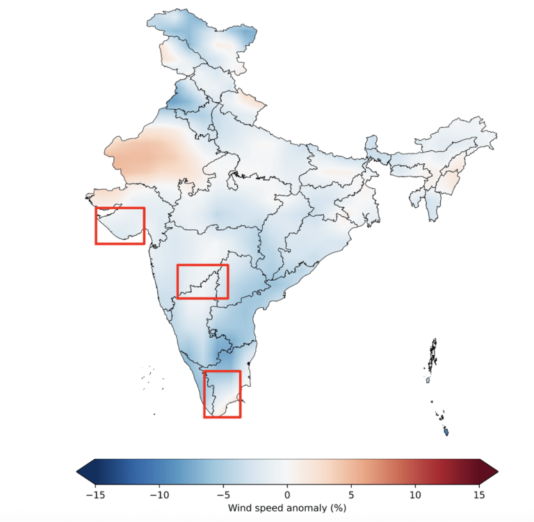
Fig 1. Multi-model wind speed anomaly (ensmean) for India. In red, the regions to focus on. Baseline period: 1993-2016.
Here, we can see the areas of relatively high wind speed anomaly are given by a red color, and the areas of relatively low wind speed anomaly are given by a blue color.
This plot indicates the expected wind speed anomaly for all of India, but again, this tells us nothing about how likely we are to actually see these values. For this, we will turn our attention to Figure 2, where a plot of the probability of finding an ensemble member in one of the three buckets of interest.
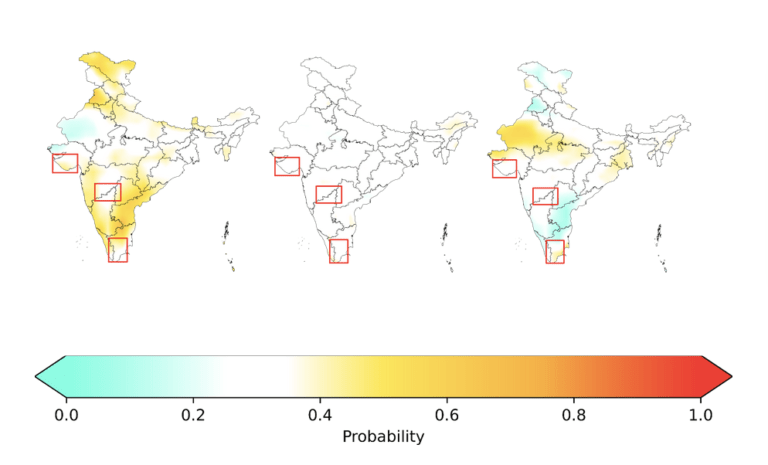

Fig 2. Multi-model probability. From left to right: low, normal & high wind probabilities. Baseline period: 1993-2016.
Now, let us focus on the three regions. Apart from a specific analysis, below the forecasts initialized in April are compared with those initialized in March and also valid by the end of April:
- Region 1 (composed by north of Karnataka, south east of Maharashtra & west Telangana)
- The members are quite evenly distributed across the terciles in the center of the region. There is a signal in the bottom left indicating a less windy month in the southeast corner of the region and a slight signal for a less windy month in the west of the region.
- This compares with last month, which showed a slight signal for a less windy month in the southeast part of the region.
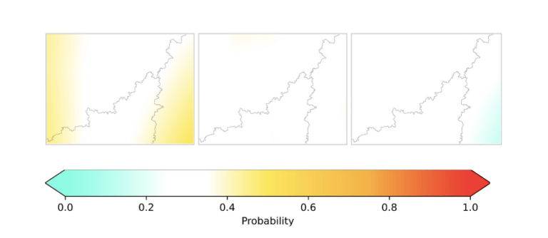
Fig 3. Multi-model probabilities for region 1 (from left to right: probability of having less, average & more wind).
- Region 2 (composed by north of Gujarat)
- There is a small probability that there will be a slightly less windy month in the south of the region and a slightly more windy month in the north of the region.
- This compares with last month’s prediction that there would be a slightly less windy month in the northeast part of the region. The model seems to have lost confidence in this prediction and has updated its prediction to be less windy in the south of the region.
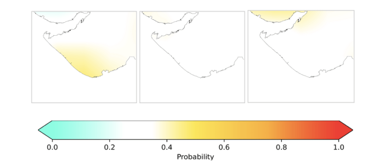
Fig 4. Multi-model probabilities for region 2 (from left to right: probability of having less, average & more wind).
- Region 3 (composed by east of Kerala & west of Tamil Nadu)
- The north of the region exhibits a strong signal that there will be a low wind month. This matches what last month’s prediction for this region was. There is also a fairly strong signal in the southeast part of the region for a windier month.
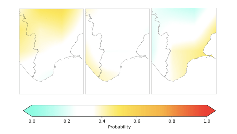
Fig 5. Multi-model probabilities for region 3 (from left to right: probability of having less, average & more wind).
Forecast for May 2025: lead month 2
Looking at the anomaly ensmean plot for the month of May, as shown in Figure 6, we can continue our analysis. There is a general prediction of normal to high anomaly for the regions of interest. If we turn our attention to the probability plots in Figure 7, we can investigate the confidence of these values.
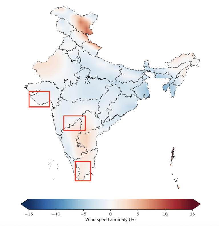
Fig 6. Multi-model wind speed anomaly (ensmean) for India. In red, the regions to focus on. Baseline period: 1993-2016
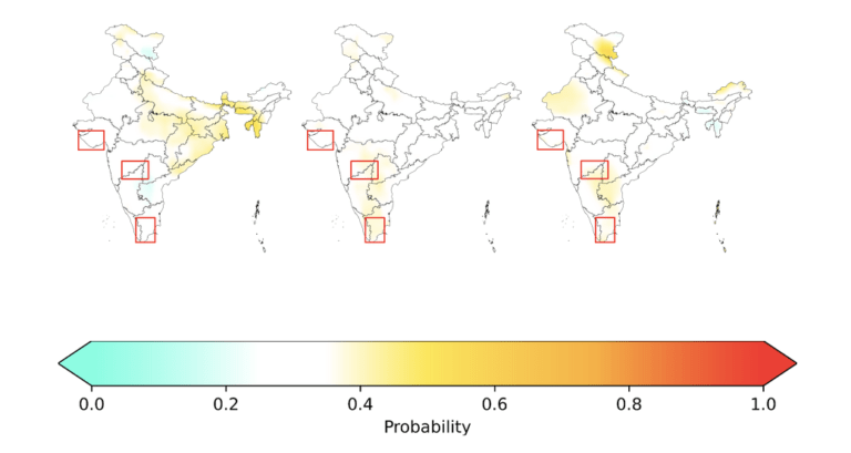
Fig 7. Multi-model probability. From left to right: low, normal & high wind probabilities. Baseline period: 1993-2016.
Now, if we focus on the three regions, we can notice:
- Region 1 (composed by north of Karnataka, south east of Maharashtra & west Telangana)
- The probabilities are quite evenly distributed across the terciles, but there is a slightly higher signal for the normal and higher terciles.
- In comparison to last month’s predictions, we see that the model has become a bit more uncertain about the wind speeds, but it is still not showing a strong signal for the low wind speed.
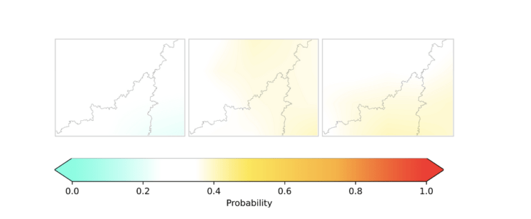
Fig 8. Multi-model probabilities for region 1 (from left to right: probability of having less, average & more wind).
- Region 2 (composed by north of Gujarat)
- Here, we see that the ensemble members are quite evenly distributed across the entire region and the model is not sure about what kind of anomaly will happen in this region.
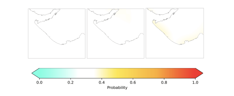
Fig 9. Multi-model probabilities for region 2 (from left to right: probability of having less, average & more wind).
- Region 3 (composed by east of Kerala & west of Tamil Nadu)
- Here, there is a fairly even spread between the normal and high anomaly buckets. There is still the stronger signal in the south of the region that there will be a slightly windier month, similar to last month’s prediction.
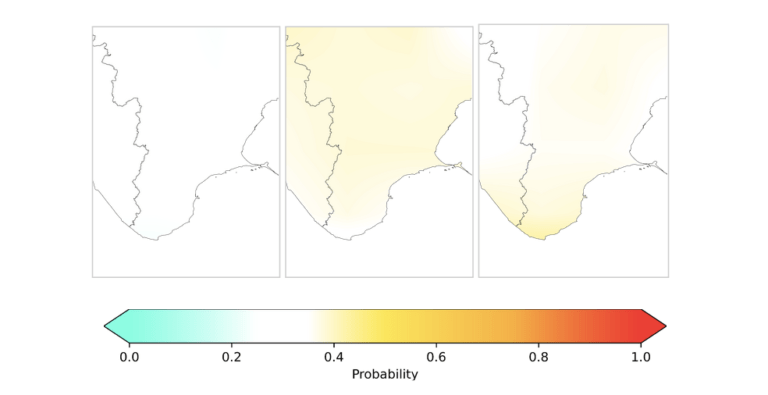
Fig 10. Multi-model probabilities for region 3 (from left to right: probability of having less, average & more wind).
Forecast for June 2025: lead month 3
Again, we will look at the anomaly ensmean and probability plots to understand what the wind speeds will look like in our regions of interest.
Looking at the anomaly ensmean plot in Figure 11, there appears to be normal wind speeds in regions 2 and 3, but a slightly higher than normal wind speed for region 1.
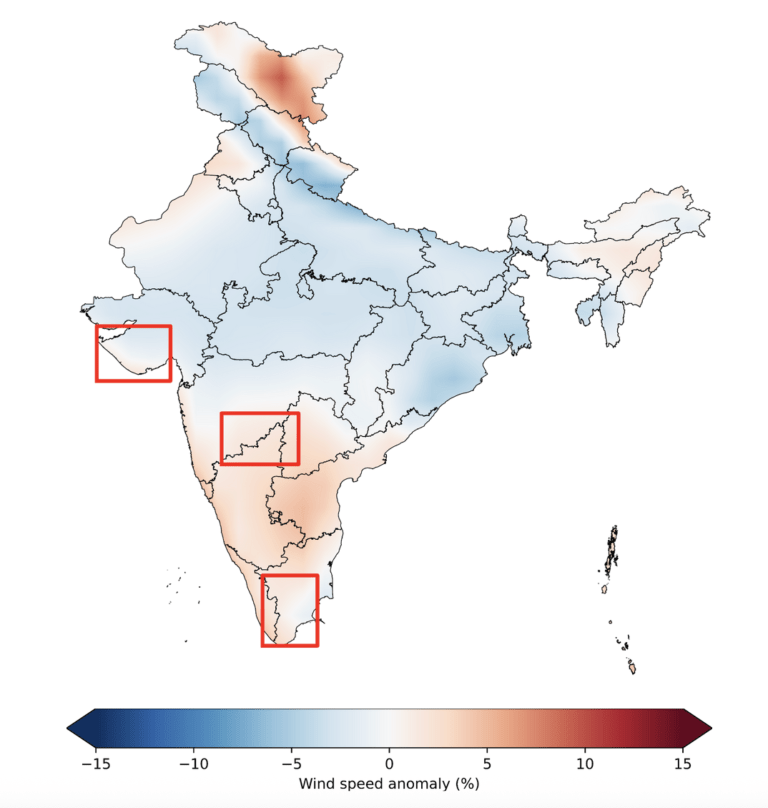
Fig 11. Multi-model wind speed anomaly (ensmean) for India. Baseline period: 1993-2016.
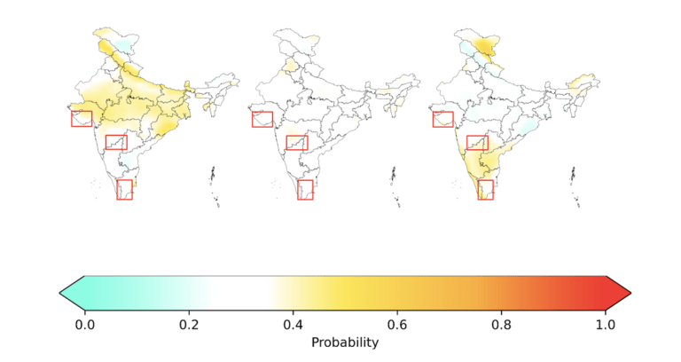
Fig 12. Multi-model probability. From left to right: low, normal & high wind probabilities. Baseline period: 1993-2016.
Now, if we focus on the three regions, we can notice:
- Region 1 (composed by north of Karnataka, south east of Maharashtra & west Telangana)
- There is a signal indicating that there will be a windier month in the southern half of the region.
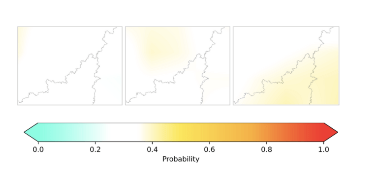
Fig 13. Multi-model probabilities for region 1 (from left to right: probability of having less, average & more wind).
- Region 2 (composed by north of Gujarat)
- There is a moderate probability of low winds in the northern half of the region, and higher winds in the southern part of the region.
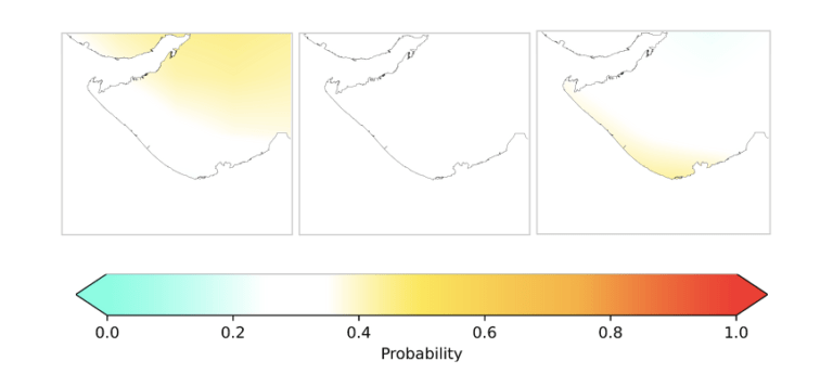
Fig 14. Multi-model probabilities for region 2 (from left to right: probability of having less, average & more wind).
- Region 3 (composed by east of Kerala & west of Tamil Nadu)
- There is a fairly strong signal that there will be a high wind anomaly in the south western part of the region, but there is good evidence that there will be high winds in most of the west part of the region. There is also some evidence that there will be lower wind speeds in the east part of the region. Everywhere else, the ensemble members are evenly distributed.
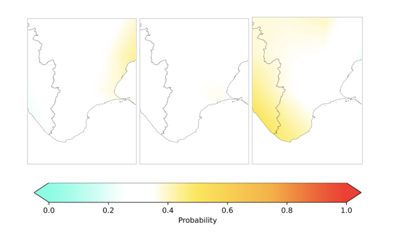
Fig 15. Multi-model probabilities for region 3 (from left to right: probability of having less, average & more wind).
Summary
In this analysis, we have explored the upcoming wind conditions in India for the months of April, May and June. The data suggests a transition from less windy conditions in April to potentially stronger winds in May and June. We have used anomaly maps to illustrate the deviations from typical wind patterns and probability maps to assess the likelihood of various wind scenarios. Understanding these techniques and how to interpret the probabilistic forecasts is crucial for preparing for the changing wind dynamics, and in this post we have shown two methods on how to do that.
